Machine learning with autoML
Data Sampling
For this classification task, we need to split the dataset into train and test sets so we can evaluate the model using the test set. We use a stratified sampling technique so that we can have equal proportion of each class in the samples. We use the createdataPartition function from the caret package to split the dataset in the ratio 75:25. We also set seed for reproducability of results.
# AutoML (Setting up connection cluster)
h2o.init()
Connection successful!
R is connected to the H2O cluster:
H2O cluster uptime: 10 hours 32 minutes
H2O cluster timezone: Africa/Lagos
H2O data parsing timezone: UTC
H2O cluster version: 3.40.0.1
H2O cluster version age: 1 month and 23 days
H2O cluster name: H2O_started_from_R_DELL_PC_puv465
H2O cluster total nodes: 1
H2O cluster total memory: 3.84 GB
H2O cluster total cores: 8
H2O cluster allowed cores: 8
H2O cluster healthy: TRUE
H2O Connection ip: localhost
H2O Connection port: 54321
H2O Connection proxy: NA
H2O Internal Security: FALSE
R Version: R version 4.2.3 (2023-03-15 ucrt) h2o.no_progress()
# Splitting the dataset into train and test sets
set.seed(1)
sampleSplit<- createDataPartition(df$PCR_outcome, p = .75, list = F)
train<- as.h2o(df[sampleSplit,])
test<- as.h2o(df[-sampleSplit,])Data Modelling
The h2o package contains a function called autoML. This autoML function automatically computes different machine learning algorithms and evaluates the best model. (LeDell and Poirier 2020)
y <- "PCR_outcome"
x <- setdiff(names(train), y)

# Run AutoML for 20 base models
aml <- h2o.automl(x = x, y = y,
                  training_frame = train,
                  max_models = 20,
                  seed = 1)
09:05:32.181: AutoML: XGBoost is not available; skipping it.
09:05:32.185: _train param, Dropping bad and constant columns: [Patient_ID]
09:05:33.35: _train param, Dropping bad and constant columns: [Patient_ID]
09:05:35.1: _train param, Dropping bad and constant columns: [Patient_ID]
09:05:38.678: _train param, Dropping bad and constant columns: [Patient_ID]
09:05:40.66: _train param, Dropping bad and constant columns: [Patient_ID]
09:05:41.637: _train param, Dropping bad and constant columns: [Patient_ID]
09:05:43.443: _train param, Dropping bad and constant columns: [Patient_ID]
09:05:47.554: _train param, Dropping bad and constant columns: [Patient_ID]
09:05:48.962: _train param, Dropping bad and constant columns: [Patient_ID]
09:45:40.674: _train param, Dropping unused columns: [Patient_ID]
09:45:42.509: _train param, Dropping unused columns: [Patient_ID]
The report of the autoML leader-board shows that the stacked Ensemble model performs the best in accurately classifying PCR_outcome with over 90% accuracy.
model_id auc logloss
1 StackedEnsemble_AllModels_1_AutoML_4_20230401_90532 0.7352096 0.4052149
2 StackedEnsemble_BestOfFamily_1_AutoML_4_20230401_90532 0.7325649 0.4074365
3 GBM_1_AutoML_4_20230401_90532 0.7324506 0.4081944
4 GBM_grid_1_AutoML_4_20230401_90532_model_3 0.7296869 0.4103241
5 GBM_grid_1_AutoML_4_20230401_90532_model_2 0.7278846 0.4100425
6 GBM_2_AutoML_4_20230401_90532 0.7228095 0.4139925
7 GBM_3_AutoML_4_20230401_90532 0.7227351 0.4135262
8 GBM_4_AutoML_4_20230401_90532 0.7217431 0.4149943
9 GBM_5_AutoML_4_20230401_90532 0.7210014 0.4151169
10 GBM_grid_1_AutoML_4_20230401_90532_model_4 0.7188969 0.4165286
aucpr mean_per_class_error rmse mse
1 0.9058269 0.3943865 0.3512496 0.1233763
2 0.9052282 0.3869225 0.3523096 0.1241221
3 0.9068157 0.4038243 0.3531263 0.1246982
4 0.9084738 0.4093145 0.3543733 0.1255804
5 0.9011726 0.4130204 0.3539831 0.1253040
6 0.8985044 0.4045695 0.3555547 0.1264191
7 0.8996143 0.4160921 0.3550859 0.1260860
8 0.9013623 0.4013015 0.3557981 0.1265923
9 0.8951907 0.4111053 0.3561440 0.1268386
10 0.9002794 0.4233731 0.3565422 0.1271223
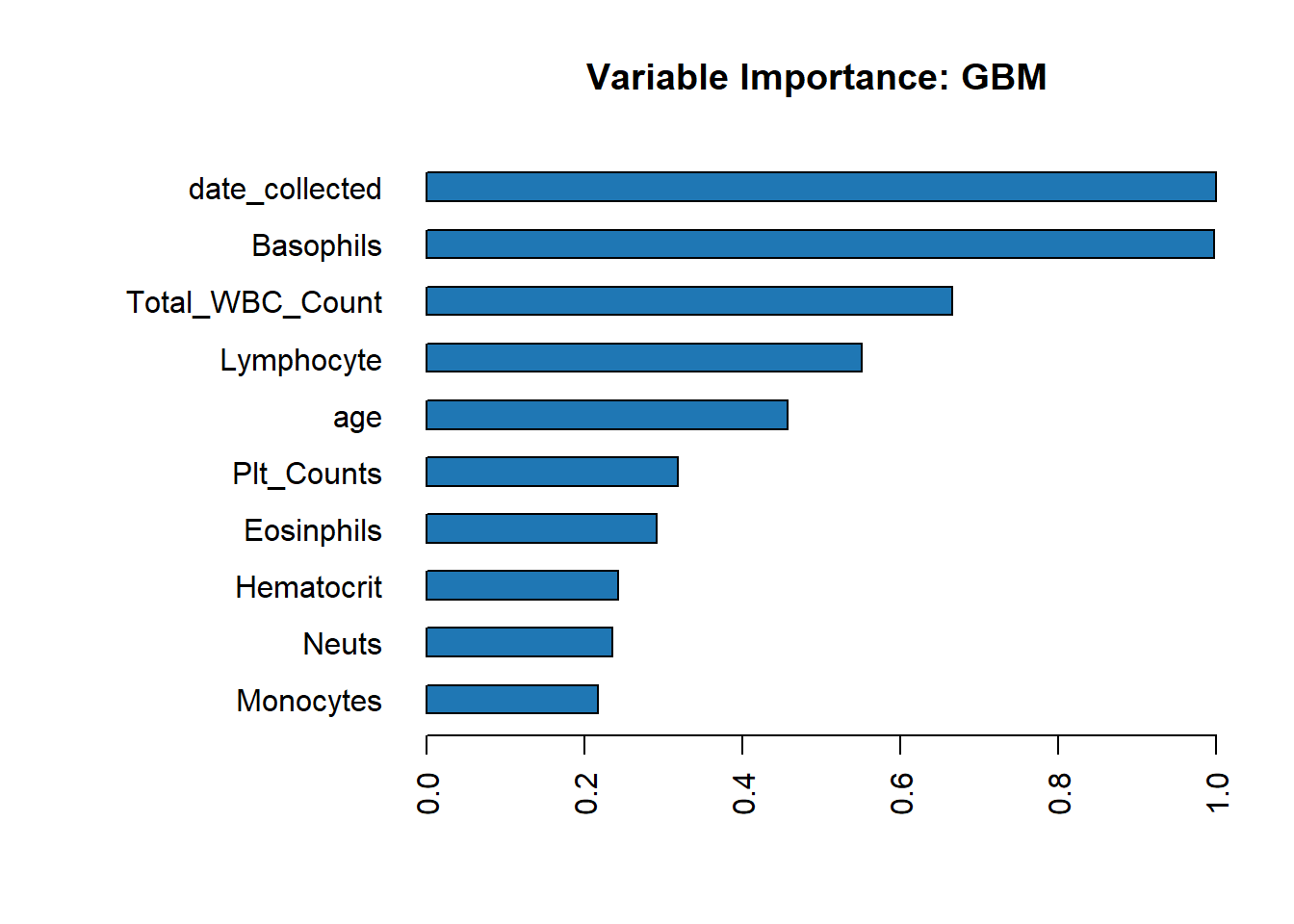
[22 rows x 7 columns] Variable Importance
Because there is no available method to obtain feature importance for the Stacked Ensemble model, we evaluate feature importance for Gradient Boosting Model (the second best model in the leader-board).
Model Evaluation
We evaluate the model using the test set. The result below shows the performance of the model.
Confusion Matrix and Statistics

              Reference
Prediction     Detected Not Detected
  Detected           73           35
  Not Detected      226         1307

               Accuracy : 0.841
                 95% CI : (0.8223, 0.8583)
    No Information Rate : 0.8178
    P-Value [Acc > NIR] : 0.007497

                  Kappa : 0.2901

 Mcnemar's Test P-Value : < 2.2e-16

            Sensitivity : 0.24415
            Specificity : 0.97392
         Pos Pred Value : 0.67593
         Neg Pred Value : 0.85258
             Prevalence : 0.18221
         Detection Rate : 0.04449
   Detection Prevalence : 0.06581
      Balanced Accuracy : 0.60903

       'Positive' Class : Detected
Conclusion and recommendations
In this report, we have been able to reach the objectives. We were able to visually explore the dataset, sample the data appropriately, model the data and evaluate the model. The Stacked ensemble model was able to outperform other models with high accuracy.
If we want outright high model performance with minimal interpretability, we may employ the stacked ensemble model but if we want a model with good performance and with more interpretable outputs, we may employ the Gradient boosting model (GBM).